Neural Network Architecture

In the previous tutorial, we learnt how a neural network works on a high level. In particular, we said that a neural network is a function like the function \(y=ax+b\) that transforms some input \(x\) into some output \(y\). However, neural networks don’t simply have a linear representation, they represent complex functions that compute arbitrary relationships. In this tutorial we will see how this works.

Brief Refresh of Linear Algebra

Linear algebra is a core concept in computer science. In general, when we want to multiply lots of numbers together, we can organise them into a matrix and then use some smart computing to make the calculation much faster than it would be if we just multiplied each number one at a time. There are plenty of terms that you might encounter on your trip through neural networks however, we will just remind you of some of the basics.

A vector is a list of numbers.

# we will use a useful numerical computation library called numpy
import numpy as np

# create a numpy vector with 4 elements
vec1 = np.array([1,2,4,3])

print("Shape:", vec1.shape)
# Shape: (4,)

print("Vector:", vec1)
# Vector: [1 2 4 3]

If you want to multiply 2 vectors together and sum the result, you use a dot product. The length of the vectors must be equal.

vec1 = np.array([1,2,4,3])
vec2 = np.array([2,2,2,2])

dot_result = np.dot(vec1, vec2)

print("Shape:", dot_result.shape)
# Shape: ()

print("Vector:", dot_result)
# Vector: 20

A matrix is a list of vectors. It has 2 dimensions: a width (how many vectors does it have) and a height (how many elements does it have in each vector).

mat1 = np.random.randn(4,3) # create a matrix with 4 rows and 3 columns
                            # with random entries

print("Shape:", mat1.shape)
# Shape: (4,3)

print("Matrix:", mat1)
# Matrix: [[ 0.87104966 -1.73364794  0.67773974]
#          [ 0.91154914 -1.59288741  0.59939096]
#          [ 0.1428397   2.05232364  1.11564538]
#          [ 0.30141196  1.91262167  0.00888209]]

Similarly, you can multiply matrices together by applying a dot product to every vector in the matrix. The vectors that are to be multiplied must have the same length. There are several notations in numpy for multiplying matrices together.

mat1 = np.random.randn(4,3) # shape (4,3)
mat2 = np.random.randn(3,4) # shape (3,4)

# The following are all equivalent
matmul1 = mat1 @ mat2 # The @ operator performs a matrix multiplication in python >=3.5
matmul2 = np.dot(mat1, mat2) # The np.dot method also performs matrix multiplication
matmul3 = np.matmul(mat1, mat2) # np.matmul is a specialised operator just for matrices

print(np.all(matmul1 == matmul2))
# True

print(np.all(matmul1 == matmul3))
# True

print("Shape:", matmul1.shape, matmul2.shape, matmul3.shape)
# Shape: (4,4) (4,4) (4,4)

Neural Networks

When we have a neural network, we usually have not just a single input \(x\). Furthermore, our parameters \(a\) and \(b\) can be also much larger than a single parameter. In fact, they are usually matrices that are multiplied with a vector input to get the output.

Lets change notation a bit: instead of a function \(y = ax+b\), we will now have a function \(y = Wx + b\). Matrices are commonly represented by capital letters and thus our parameter \(W\) is now a matrix. This matrix is called a weight matrix. Similarly, \(x\) and \(b\) are now vectors so that they can be multiplied and added to the weight matrix respectively. The vector \(b\) is called the bias as it moves the linearity up and down on the y axis. The shape of the vector \(y\) can be inferred by the shape of \(W\) - we can have a prediction for a single label or for many labels.

W = np.random.randn(10,2)
x = np.random.randn(10)
b = np.ones(2)

y = np.dot(x, W) + b
print(y.shape)
# (2,)

However, the function \(y = Wx + b\) is a linear function and thus cannot generalise to arbitrary functions - we want something more powerful. What we do to vary the function in a non-linear way is apply some sort of non-linearity function, which are also called activation functions. These functions can have various shapes but one of the most popular is the Rectified Linear Unit (ReLU) function. It takes its input and makes all negative numbers 0 while leaving positive numbers alone. It looks like this:

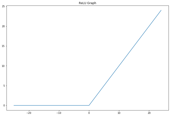
A ReLU in code would look like this:

relu_out = np.maximum(x, 0) # take the maximum between x and 0

Furthermore, we want to use many layers of computation in order to calculate complex dependencies in our data. This leads us to deep neural networks. Also it’s important to note that without the ReLU non-linearity, any cascaded linear layers would combine resulting in the effect of a single linear layer because of linearity. Now we can cascade linear layers and ReLU activation functions in this manner: Linear -> ReLU -> Linear -> ReLU -> Linear -> Output. The lack of a ReLU after the last linear layer is because the outputs of the last layer are our predictions and we don’t want to arbitrarily mess with them.

This basic pattern leads to the image you’ll see whenever someone talks about a neural network:

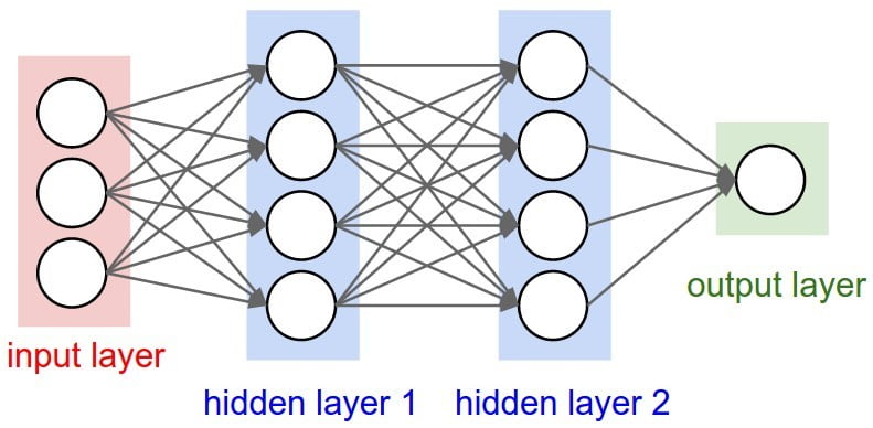Image from here.

The lines represent the weights and the circles represent the activation functions. You can see that we can combine many of these layers together to create deep networks. Finally you can also see how the input and output can be any shape.

In the next tutorial, we learn how to use a popular machine learning framework called PyTorch to build and train neural networks.